Attention Is All You Need

Vaswani et al. · NIPS 2017 · arXiv:1706.03762

Ashish Vaswani Noam Shazeer Niki Parmar Jakob Uszkoreit Llion Jones Aidan N. Gomez Łukasz Kaiser Illia Polosukhin

📅 Published: June 2017 (v7: Aug 2023) 🏢 Google Brain / Google Research 📍 NIPS 2017, Long Beach, CA 🔗 arxiv.org/abs/1706.03762 💻 tensor2tensor on GitHub

🌟 Why This Paper Matters

This single paper introduced the Transformer architecture — the foundation of every modern LLM including GPT-4, Claude, Gemini, and LLaMA. Understanding it is essential for any AI engineer.

Abstract

The dominant sequence transduction models are based on complex recurrent or convolutional neural networks that include an encoder and a decoder. The best performing models also connect the encoder and decoder through an attention mechanism. We propose a new simple network architecture, the Transformer, based solely on attention mechanisms, dispensing with recurrence and convolutions entirely. Experiments on two machine translation tasks show these models to be superior in quality while being more parallelizable and requiring significantly less time to train. Our model achieves 28.4 BLEU on the WMT 2014 English-to-German translation task, improving over the existing best results, including ensembles, by over 2 BLEU. On the WMT 2014 English-to-French translation task, our model establishes a new single-model state-of-the-art BLEU score of 41.8 after training for 3.5 days on eight GPUs, a small fraction of the training costs of the best models from the literature.

Key Numbers at a Glance

28.4

BLEU — EN→DE (SOTA)

41.8

BLEU — EN→FR (SOTA)

3.5

Days to train (8× P100)

Attention heads (base)

512

d_model (base)

Encoder / Decoder layers

65M

Parameters (base)

3.3×10¹⁸

FLOPs to train (base)

1. Introduction

Prior to the Transformer, the dominant approaches to sequence modeling were recurrent neural networks (RNNs) — specifically LSTMs and GRUs. These models process sequences token-by-token, maintaining a hidden state that is updated at each step.

⚠ The Problem with RNNs

Sequential computation prevents parallelization. Hidden state h_t depends on h_t-1, so you cannot process position 10 until positions 1–9 are done. This becomes a critical bottleneck at long sequence lengths.

Attention mechanisms were already used alongside RNNs to handle long-range dependencies without regard to distance. But they were always used in conjunction with a recurrent architecture.

💡 The Key Insight

The Transformer proposes using attention mechanisms alone — dispensing with recurrence and convolutions entirely. This enables full parallelization and achieves state-of-the-art quality with far less training time.

2. Background

Earlier attempts to reduce sequential computation used convolutional neural networks (ByteNet, ConvS2S). In those models, the number of operations to relate two positions grows with their distance — linearly for ConvS2S, logarithmically for ByteNet.

Self-attention (intra-attention) relates different positions of a single sequence to compute a representation. It had been used in reading comprehension, summarization, and textual entailment tasks.

ℹ️ Key Claim

The Transformer is the first transduction model relying entirely on self-attention to compute its input/output representations — without sequence-aligned RNNs or convolutions.

3. Model Architecture

The Transformer follows the standard encoder-decoder structure. The encoder maps input (x₁, …, xₙ) to continuous representations z = (z₁, …, zₙ). The decoder generates output (y₁, …, yₘ) one element at a time, auto-regressively.

Figure 1: The Transformer model architecture — encoder (left, blue) and decoder (right, purple) each composed of 6 identical layers.

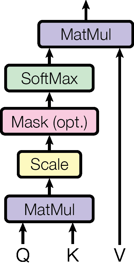
Complete Transformer architecture with encoder and decoder stacks

Figure 1b: Full Transformer architecture in detail — showing encoder (left) and decoder (right) with Nx repetition of identical layers, input/output embeddings, positional encoding, and cross-attention connections.

3.1 Encoder and Decoder Stacks

🔵

Encoder

Stack of N=6 identical layers. Each has: (1) Multi-head self-attention, (2) Position-wise FFN. Both wrapped with residual connection + LayerNorm. All sub-layers output d_model=512.

🟣

Decoder

Stack of N=6 identical layers. Each has: (1) Masked self-attention, (2) Cross-attention over encoder output, (3) Position-wise FFN. Masking prevents attending to future positions.

💡 Residual Connections

Every sub-layer computes LayerNorm(x + Sublayer(x)). The residual connection allows gradients to flow unchanged through the network, enabling training of deep stacks.

3.2 Attention

An attention function maps a query and a set of key-value pairs to an output. The output is a weighted sum of values, where weights come from the compatibility of the query with each key.

3.2.1 Scaled Dot-Product Attention

Attention(Q, K, V) = softmax( QKᵀ / √d_k ) · V

Equation (1) — Scaled Dot-Product Attention

Queries and keys have dimension d_k; values have dimension d_v. The scaling factor 1/√d_k prevents the dot products from growing large (which would push the softmax into regions with very small gradients).

⚠ Why Scale by √d_k?

Assume components of q and k are i.i.d. with mean 0, variance 1. Then q·k = Σ qᵢkᵢ has mean 0 but variance d_k. Scaling brings variance back to 1, keeping softmax gradients healthy.

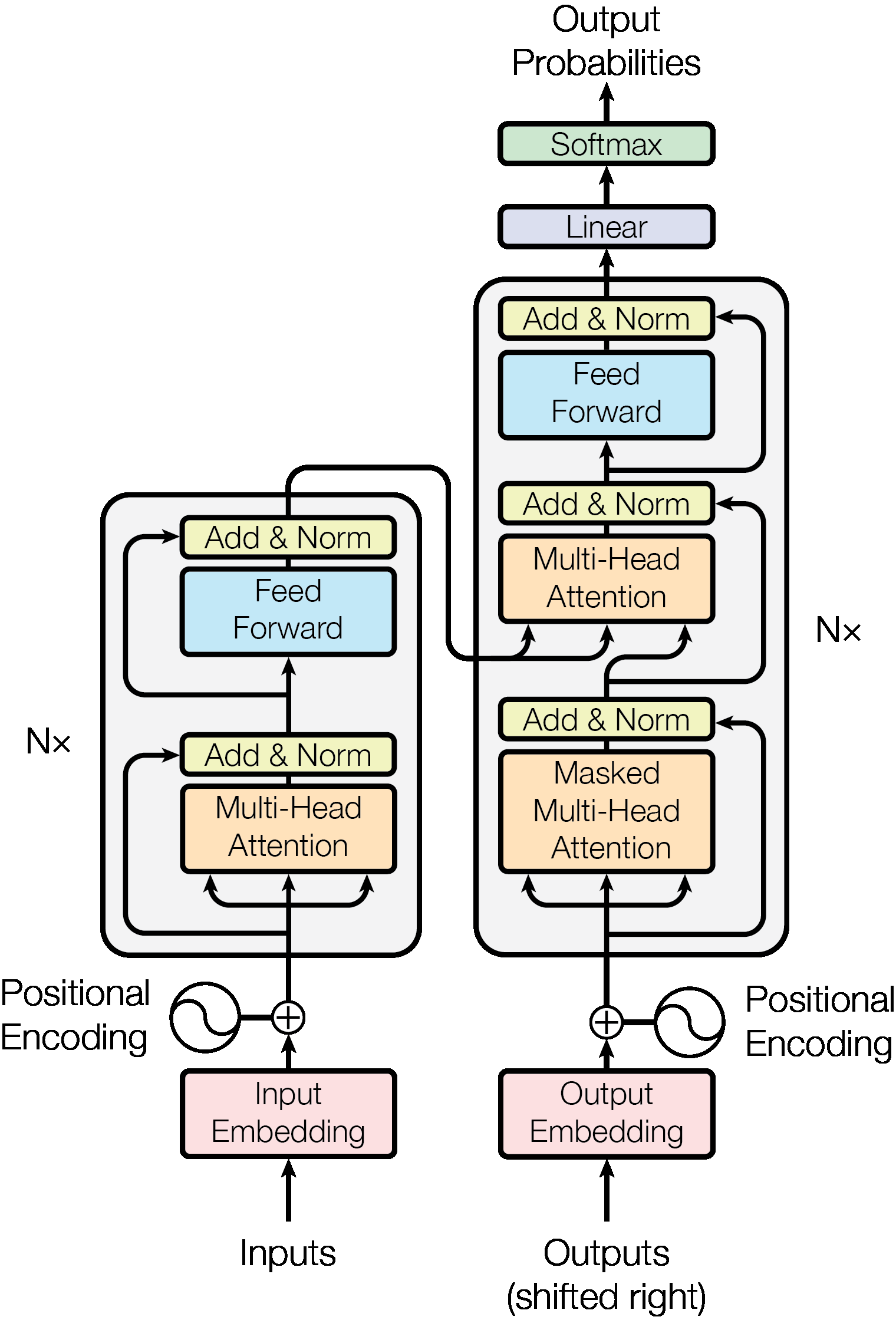
Scaled Dot-Product Attention mechanism diagram

Figure 2: Scaled Dot-Product Attention — the core building block. Queries (Q), Keys (K), and Values (V) flow through MatMul, Scale, Mask, SoftMax, and MatMul to produce attention-weighted output.

3.2.2 Multi-Head Attention

Instead of one large attention function, project queries, keys and values h times with different learned linear projections, run attention in parallel, then concatenate.

MultiHead(Q,K,V) = Concat(head₁, …, head_h) W^O
where head_i = Attention(QW^Q_i, KW^K_i, VW^V_i)

Equation — Multi-Head Attention

💡 Why Multiple Heads?

Each head can attend to information from different representation subspaces at different positions. A single attention head averaging over all positions inhibits this. In the base model: h=8, d_k=d_v=64.

Multi-Head Attention mechanism showing concatenation of attention heads

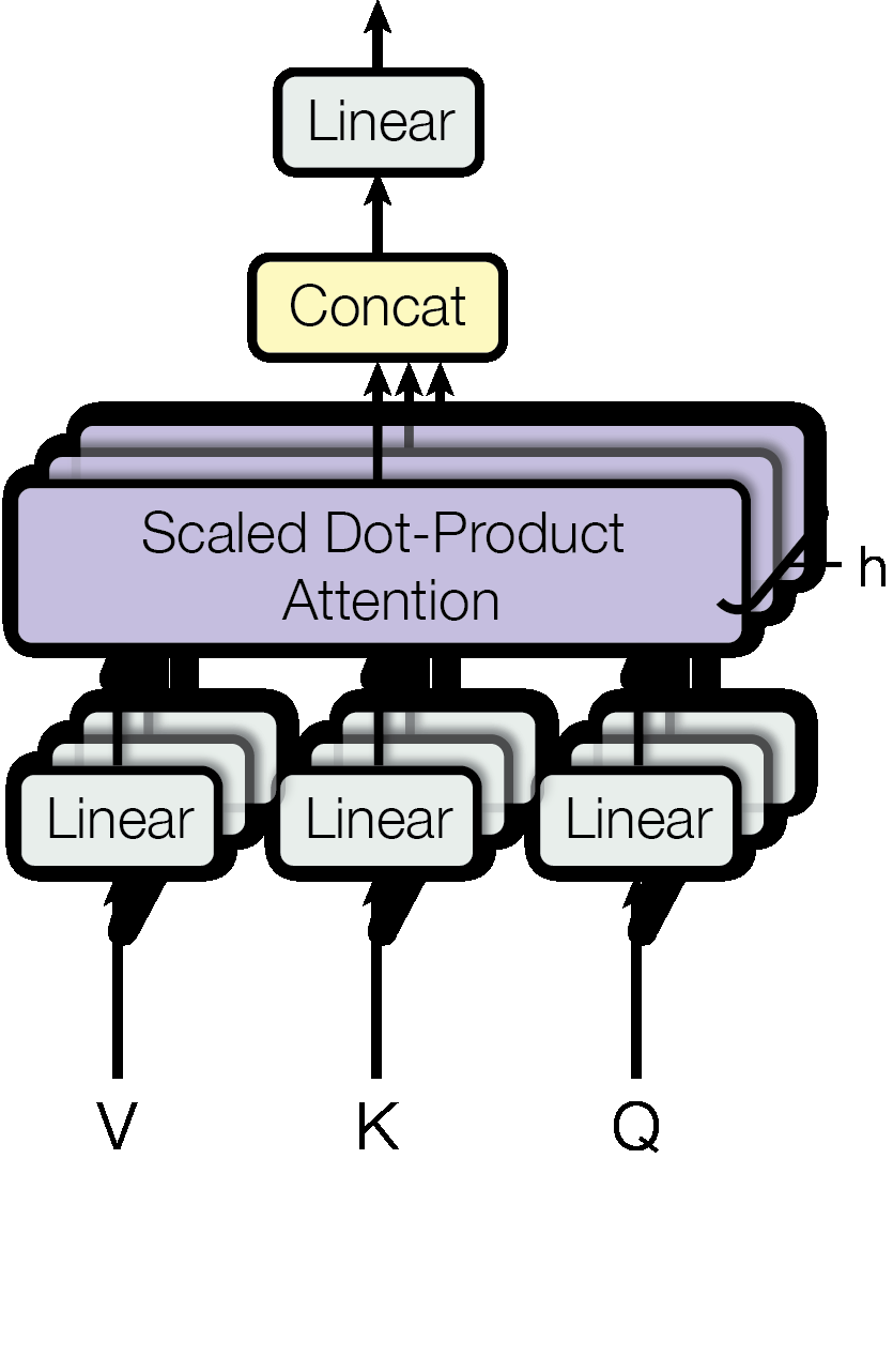
Figure 3: Multi-Head Attention — multiple attention heads (shown as parallel operations) process the input independently, then their outputs are concatenated and passed through a final linear layer.

3.2.3 Applications of Attention in the Transformer

Encoder self-attention: Each encoder position attends to all positions in the previous encoder layer.
Decoder masked self-attention: Each decoder position attends to all positions up to and including itself (future positions masked with −∞).
Encoder-decoder (cross) attention: Decoder queries attend over all encoder output positions — the keys and values come from the encoder.

3.3 Position-wise Feed-Forward Networks

Each encoder/decoder layer contains a fully connected FFN applied identically to each position:

FFN(x) = max(0, xW₁ + b₁)W₂ + b₂

Equation (2) — Two linear transformations with ReLU between them

d_model=512 on input/output; inner layer d_ff=2048.

3.4 Embeddings and Softmax

Learned embeddings convert tokens to d_model-dimensional vectors. The same weight matrix is shared between: the two embedding layers and the pre-softmax linear transformation. Embedding weights are multiplied by √d_model.

3.5 Positional Encoding

Since the Transformer has no recurrence or convolution, it has no inherent sense of token order. Positional encodings are added to input embeddings at the bottom of both encoder and decoder stacks.

PE(pos, 2i) = sin(pos / 10000^2i/d_model)
PE(pos, 2i+1) = cos(pos / 10000^2i/d_model)

Sinusoidal positional encoding — each dimension is a sinusoid of different frequency

ℹ️ Why Sinusoids?

For any fixed offset k, PE_pos+k can be represented as a linear function of PE_pos. This lets the model easily learn to attend by relative positions. Also, sinusoidal encodings can extrapolate to longer sequences than seen during training.

4. Why Self-Attention

Three motivating criteria for preferring self-attention over recurrent and convolutional layers:

Layer Type	Complexity per Layer	Sequential Ops	Max Path Length
Self-Attention	O(n² · d)	O(1)	O(1)
Recurrent	O(n · d²)	O(n)	O(n)
Convolutional	O(k · n · d²)	O(1)	O(log_k(n))
Self-Attn (restricted)	O(r · n · d)	O(1)	O(n/r)

🔑 Key Insight

Self-attention connects all positions with O(1) sequential operations. For typical sentence-level tasks where n < d, self-attention is also faster than recurrent layers per-layer. The O(n²) complexity is manageable for typical NLP sequence lengths.

5. Training

📦

Data

WMT 2014 EN-DE: ~4.5M sentence pairs (37K token BPE vocab). WMT 2014 EN-FR: 36M sentences (32K wordpiece vocab).

🖥️

Hardware

8× NVIDIA P100 GPUs. Base model: 0.4s/step, 100K steps (~12 hours). Big model: 1.0s/step, 300K steps (3.5 days).

📐

Optimizer

Adam (β₁=0.9, β₂=0.98, ε=10⁻⁹). Warmup for 4000 steps then inverse square root decay.

🛡️

Regularization

Residual dropout P_drop=0.1. Label smoothing ε_ls=0.1 (hurts perplexity but improves BLEU).

lrate = d_model^−0.5 · min(step_num^−0.5, step_num · warmup_steps^−1.5)

Equation (3) — Learning rate schedule: linear warmup, then inverse sqrt decay

6. Results

6.1 Machine Translation

28.4

BLEU on EN→DE

+2 BLEU over all prior models including ensembles

41.8

BLEU on EN→FR

New single-model SOTA at <¼ the training cost

3.3×10¹⁸

FLOPs (base model)

vs 2.3×10¹⁹ for GNMT+RL, a 7× reduction

Model	EN-DE BLEU	EN-FR BLEU	EN-DE FLOPs	EN-FR FLOPs
GNMT + RL	24.6	39.92	2.3×10¹⁹	1.4×10²⁰
ConvS2S	25.16	40.46	9.6×10¹⁸	1.5×10²⁰
MoE	26.03	40.56	2.0×10¹⁹	1.2×10²⁰
ConvS2S Ensemble	26.36	41.29	7.7×10¹⁹	1.2×10²¹
Transformer (base)	27.3	38.1	3.3×10¹⁸	—
Transformer (big)	28.4	41.8	2.3×10¹⁹	—

6.2 Model Variations (Ablations)

Key findings from ablation experiments (Table 3 in the paper):

Attention heads: Single-head attention is 0.9 BLEU worse than h=8. But too many heads also hurts.
Key dimension d_k: Reducing d_k hurts quality — dot-product compatibility is non-trivial.
Bigger models are better and dropout is critical for avoiding overfitting.
Positional encoding: Learned embeddings yield nearly identical results to sinusoidal — but sinusoidal can generalize to longer sequences.

6.3 English Constituency Parsing

To test generalization, the authors trained a 4-layer Transformer (d_model=1024) on the WSJ Penn Treebank (~40K sentences).

✅ Result

Transformer achieves 92.7 F1 in semi-supervised setting — outperforming all prior models except the Recurrent Neural Network Grammar, with no task-specific tuning.

7. Conclusion

The Transformer is the first sequence transduction model based entirely on attention, replacing recurrent layers with multi-headed self-attention. Key advantages:

Significantly faster to train than RNN/CNN architectures
Achieves new SOTA on EN-DE and EN-FR translation
Generalizes to other tasks (constituency parsing) without task-specific modifications

🚀 Legacy

This architecture became the foundation for BERT (2018), GPT (2018), T5 (2019), and every modern LLM. Virtually every state-of-the-art model in NLP, vision, audio, and multimodal AI is now built on the Transformer.

Review Questions

Why does standard RNN processing prevent parallelization, and how does the Transformer solve this?
Derive the scaling factor 1/√d_k from the variance argument. What happens without it?
What is the difference between encoder self-attention, decoder self-attention, and cross-attention?
Why does the paper prefer sinusoidal positional encodings over learned embeddings?
In Table 1 of the paper, self-attention has O(n²·d) complexity per layer. When does this become worse than recurrent layers?
What is label smoothing and why does it hurt perplexity but improve BLEU?
The paper uses beam search at inference. What is beam size and how does it trade off quality vs. speed?